Saturday, May 20, 2017

Yahoo is dead, long live Yahoo!

On 18 May 2017 the ichart data api of yahoo finance went down, without any notice. And it does not seem like it is coming back. This has left many (including me) with broken code and without a descent free end-of-day data source. Something needs to be done. Now.

Apparently Yahoo! does not want us to download free data automatically, but it is still possible to download it by hand, clicking the 'download' button on the ticker webpage. Automatic downloading is made more difficult by using a cookie-crub pair, but luckily still possible.

I'm now working on updating the tradingWithPython.yahooFinance library and as a part of that work I've created a proto script that shows how to get the data. Because so many are now  scrambling to get their code working, I'm sharing this as soon as possible.

The notebook can be found on Github, enjoy!

Update: yahooFinance.py has been fixed!


Note: the data provided seems to be adjusted for splits, but not for dividends.

Saturday, February 20, 2016

A simple statistical edge in SPY

I've recently read a great post by the turinginance blog on how to be a quant.  In short, it describes a scientific approach to developing trading strategies. For me personally, observing data, thinking with models and forming hypothesis is a second nature, as it should be for any good engineer.

In this post I'm going to illustrate this approach by explicitly going through a number of steps (just a couple, not all of them) involved in development of a trading strategy.

Let's take a look at the most common trading instrument, the S&P 500 ETF  'SPY' . I'll start with observations.

Observations
It occurred to me that most of the time that there is much talk in the media about the market crashing (after big losses over several days timespan), quite a significant rebound sometimes follows.
In the past I've made a couple of mistakes by closing my positions to cut losses short, just to miss out a recovery in the following days.

General theory
After a period of consecutive losses, many traders will liquidate their positions out of fear for even larger loss. Much of this behavior is governed by fear, rather than calculated risk. Smarter traders come in then for the bargains.

Hypothesis: Next-day returns of SPY will show an upward bias after a number of consecutive losses.

To test the hypothesis, I've calculated the number of consecutive 'down' days . Everything under -0.1% daily return qualifies as a 'down' day.


The return series are near-random, so as one would expect, the chances of 5 or more consecutive down days are low, resulting in a very limited number of occurrences. Low number of occurrences will result in unreliable statistical estimates, so I'll stop at 5.

Below is a visualisation of nex-tday returns as a function of number of down days.


I've also plotted 90% confidence interval of the returns between the lines. It turns out that the average return *is* positively correlated with the number of down days. Hypothesis confirmed.

However, you can clearly see that this extra alpha is very small compared to the band of the probable return outcomes. But even a tiny edge can be exploited (find a statistical advantage and repeat as often as possible). Next step is to investigate if this edge can be turned in a trading strategy.

Given the data above, a trading strategy can be forumlated:
After consectutive 3 or more losses, go long. Exit on next close.

Below is a result of this strategy compared to pure buy-and-hold.

This does not look bad at all! Looking a the sharpe ratios the strategy scores a descent 2.2 versus 0.44 for the B&H.  This is actually pretty good!  ( don't get too excited though, as I did not account for commision costs, slippage etc ).


While the strategy above is not something that I would like to trade simply because of the long time span, the theory itself provokes futher thoughts that could produce something useful. If the same principle applies to intraday data, a form of scalping strategy could be built. In the example above I've oversimplified the world a bit by only counting the *number* of down days, without paying attention to the depth of the drawdown. Also, position exit is just a basic 'next-day-close' . There is much to be improved, but the essence in my opinion is this:

future returns of SPY are ifluenced by drawdown and drawdown duration over the previous 3 to 5 days.


Monday, November 17, 2014

Trading VXX with nearest neighbors prediction

An experienced trader knows what behavior to expect from the market based on a set of indicators and their interpretation. The latter is often done based on his memory or some kind of model. Finding a good set of indicators and processing their information poses a big challenge. First, one needs to understand what  factors are correlated to future prices. Data that does not have any predictive quality only intorduces noise and complexity, decreasing strategy performance. Finding good indicators is a science on its own, often requiring deep understandig of the market dynamics. This part of strategy design can not be easily automated. Luckily, once a good set of indicators has been found, the traders memory and 'intuition' can be easily replaced with a statistical model, which will likely to perform much better as computers do have flawless memory and can make perfect statistical estimations.

Regarding volatility trading, it took me quite some time to understand what influences its movements. In particular, I'm interested in variables that predict future returns of VXX and  XIV. I will not go into full-length explanation here, but just present a conclusion : my two most valuable indicators for volatility are the term structure slope and current volatility premium.
My definition of these two is:

  • volatility premium = VIX-realizedVol
  • delta (term structure slope) = VIX-VXV
VIX & VXV are the forward 1 and 3 month implied volatilities of the S&P 500. realizedVol here is a 10-day realized volatility of SPY, calculated with Yang-Zhang formula. delta  has been often discussed on VixAndMore blog, while premium is well-known from option trading.

It makes sense to go short volatility when premium  is high and futures are in contango (delta  < 0). This will cause a tailwind from both the premium and daily roll along the term structure in VXX. But this is just a rough estimation. A good trading strategy would combine information from both premium and delta to come with a prediction on trading direction in VXX.
I've been struggling for a very long time to come up with a good way to combine the noisy data from both indicators. I've tried most of the 'standard' approaches, like linear regression, writing a bunch of 'if-thens' , but all with a very minor improvements compared to using only one indicator. A good example of such 'single indicator' strategy with simple  rules can be found on TradingTheOdds blog . Does not look bad, but what can be done with multiple indicators?

I'll start with some out-of-sample VXX data that I got from MarketSci. Note that this is simulated data, before VXX was created. 


The indicators for the same period are plotted below:


If we take one of the indicators (premium in this case) and plot it against future returns of VXX, some correlation can be seen, but the data is extremely noisy:


Still, it is clear that negative premium is likely to have positive VXX returns on the next day.
Combining both premium and delta into one model has been a challenge for me, but I always wanted to do a statistical approximation. In essence, for a combination of (delta,premium), I'd like to find all historic values that are closest to the current values and make an estimation of the future returns based on them. A couple of times I've started writing my own nearest-neighbor interpolation algorithms, but every time I had to give up... until I came across the scikit nearest neighbors regression. It enabled me to quickly build a predictor based on two inputs and the results are so good, that I'm a bit worried that I've made a mistake somewhere...

Here is what I did:

  1. create a dataset of [delta,premium] -> [VXX next day return] (in-of-sample)
  2. create a nearest-neighbor predictor based on the dataset above
  3. trade strategy (out-of-sample) with the rules:
    • go long if predicted return > 0
    • go short if predicted return <0
The strategy could not be simpler...

The results seem extremely good and get better when more neigbors are used for estimation.
First, with 10 points, the strategy is excellent in-sample, but is flat out-of-sample (red line in figure below is the last point in-sample)

Then, performance gets better with 40 and 80 points:


In the last two plots, the strategy seems to perform the same in- and out-of-sample. Sharpe ratio is around 2.3.
I'm very pleased with the results and have the feeling that I've only been scratching the surface of what is possible with this technique.


Wednesday, July 16, 2014

Simple backtesting module


My search of an ideal backtesting tool (my definition of 'ideal' is described in the earlier 'Backtesting dilemmas' posts) did not result in something that I could use right away. However, reviewing the available options helped me to understand better what I really want. Of the options I've looked at, pybacktest was the one I liked most because of its simplicity and speed. After going through the source code,  I've got some ideas to make it simpler and a bit more elegant. From there, it was only a small step to writing my own backtester, which is now available in the TradingWithPython library.

I have chosen an approach where the backtester contains functionality which all trading strategies share and that often gets copy-pasted. Things like calculating positions and pnl, performance metrics and making plots.

Strategy specific functionality, like determining entry and exit points should be done outside of the backtester. A typical workflow would be:
find entry and exits -> calculate pnl and make plots with backtester -> post-process strategy data

At this moment the module is very minimal (take a look at the source here), but in the future I plan on adding profit and stop-loss exits and multi-asset portfolios.

Usage of the backtesting module is shown in this example notebook

Saturday, June 7, 2014

Boosting performance with Cython


Even with my old pc (AMD Athlon II, 3GB ram), I seldom run into performance issues when running vectorized code. But unfortunately there are plenty of cases where that can not be easily vectorized, for example the drawdown function. My implementation of such was extremely slow, so I decided to use it as a test case for speeding things up. I'll be using the SPY timeseries with ~5k samples as test data. Here comes the original version of my drawdown function (as it is now implemented in the TradingWithPython library)
def drawdown(pnl):
    """
    calculate max drawdown and duration

    Returns:
        drawdown : vector of drawdwon values
        duration : vector of drawdown duration
    """
    cumret = pnl

    highwatermark = [0]

    idx = pnl.index
    drawdown = pd.Series(index = idx)
    drawdowndur = pd.Series(index = idx)

    for t in range(1, len(idx)) :
        highwatermark.append(max(highwatermark[t-1], cumret[t]))
        drawdown[t]= (highwatermark[t]-cumret[t])
        drawdowndur[t]= (0 if drawdown[t] == 0 else drawdowndur[t-1]+1)

    return drawdown, drawdowndur

%timeit drawdown(spy)
1 loops, best of 3: 1.21 s per loop
Hmm 1.2 seconds is not too speedy for such a simple function. There are some things here that could be a great drag to performance, such as a list *highwatermark* that is being appended on each loop iteration. Accessing Series by their index should also involve some processing that is not strictly necesarry. Let's take a look at what happens when this function is rewritten to work with numpy data
def dd(s):
#    ''' simple drawdown function '''
    
    highwatermark = np.zeros(len(s))
    drawdown = np.zeros(len(s))
    drawdowndur = np.zeros(len(s))

 
    for t in range(1,len(s)):
        highwatermark[t] = max(highwatermark[t-1], s[t])
        drawdown[t] = (highwatermark[t]-s[t])
        drawdowndur[t]= (0 if drawdown[t] == 0 else drawdowndur[t-1]+1)
       
     
    return drawdown , drawdowndur

%timeit dd(spy.values)
10 loops, best of 3: 27.9 ms per loop
Well, this is much faster than the original function, approximately 40x speed increase. Still there is much room for improvement by moving to compiled code with cython Now I rewrite the dd function from above, but using optimisation tips that I've found on the cython tutorial . Note that this is my first try ever at optimizing functions with Cython.
%%cython
import numpy as np
cimport numpy as np

DTYPE = np.float64
ctypedef np.float64_t DTYPE_t

cimport cython
@cython.boundscheck(False) # turn of bounds-checking for entire function
def dd_c(np.ndarray[DTYPE_t] s):
#    ''' simple drawdown function '''
    cdef np.ndarray[DTYPE_t] highwatermark = np.zeros(len(s),dtype=DTYPE)
    cdef np.ndarray[DTYPE_t] drawdown = np.zeros(len(s),dtype=DTYPE)
    cdef np.ndarray[DTYPE_t] drawdowndur = np.zeros(len(s),dtype=DTYPE)

    cdef int t
    for t in range(1,len(s)):
        highwatermark[t] = max(highwatermark[t-1], s[t])
        drawdown[t] = (highwatermark[t]-s[t])
        drawdowndur[t]= (0 if drawdown[t] == 0 else drawdowndur[t-1]+1)
        
    return drawdown , drawdowndur

%timeit dd_c(spy.values)
10000 loops, best of 3: 121 µs per loop

Wow, this version runs in 122 microseconds, making it ten thousand times faster than my original version! I must say that I'm very impressed by what the Cython and IPython teams have achieved! The speed compared with ease of use is just awesome!
 P.S. I used to do code optimisations in Matlab using pure C and .mex wrapping, it was all just pain in the ass compared to this.

Tuesday, May 27, 2014

Backtesting dilemmas: pyalgotrade review

Ok, moving on to the next contestant: PyAlgoTrade

First impression: actively developed, pretty good documentation, more than enough feautures ( TA indicators, optimizers etc) . Looks good, so I went on with the installation which also went smoothly.

The tutorial seems to be a little bit out of date, as the first command yahoofinance.get_daily_csv() throws an error about unknown function. No worries, the documentation is up to date and I find that the missing function is now renamed to yahoofinance.download_daily_bars(symbol,year,csvFile). The problem is that this function only downloads data for one year instead of everything from that year to current date. So pretty useless.
After I downloaded the data myself and saved it to csv, I needed to adjust the column names because apparently pyalgotrade expects Date,Adj Close,Close,High,Low,Open,Volume to be in the header. That is all minor trouble.

Following through to performance testing on an SMA strategy that is provided in the tutorial. My dataset consists of 5370 days of SPY:

%timeit myStrategy.run()
1 loops, best of 3: 1.2 s per loop

That is actually pretty good for an event-based framework.

But then I tried searching documentation for functionality needed to backtest spreads and multiple asset portfolios and just could not find any. Then I tried to find a way to feed pandas DataFrame as an input to a strategy and it happens to be not possible, which is again a big disappointment. I did not state it as a requirement in the previous post, but now I come to realisation that pandas support is a must for any framework that works with time series data. Pandas was a reason for me to switch from Matlab to Python and I never want to go back.

Conclusion pyalgotrade does not meet my requrement for flexibility. It looks like it was designed with classic TA in mind and single instrument trading. I don’t see it as a good tool for backtesting strategies that involve multiple assets, hedging etc.

Monday, May 26, 2014

Backtesting dilemmas

A quantitative trader faces quite some challenges on a way to a successful trading strategy. Here I’ll discuss a couple dilemmas involved in backtesting. A good trading simulation must :
  1. Be good approximation of the real world. This one is of course the most important requirement .
  2. Allow unlimited flexibility: the tooling should not stand in the way of testing out-of-the-box ideas. Everything that can be quantified should be usable.
  3. Be easy to implement & maintain. It is all about productivity and being able to test many ideas to find one that works.
  4. Allow for parameter scans, walk-forward testing and optimisations. This is needed for investigating strategy performance and stability depending on strategy parameters.
The problem with satisfying all of the requirements above is that #2 and #3 are conflicting ones. There is no tool that can do everything without the cost of high complexity (=low maintainablity). Typically, a third party point-and-click tool will severely limit freedom to test with custom signals and odd portfolios, while at the other end of the spectrum a custom-coded diy solution will require tens or more hours to implement with high chances of ending up with cluttered and unreadable code. So in attempt to combine the best of both worlds, let’s start somewehere in the middle: use an existing backtesting framework and adapt it to our taste.
In the following posts I’ll be looking at three possible candidates I’ve found:
  • Zipline is widely known and is the engine behind Quantopian
  • PyAlgotrade seems to be actively developed and well-documented
  • pybacktest is a light-weight vector-based framework with that might be interesting because of its simplicity and performance.
I’ll be looking at suitability of these tools benchmarking them against a hypothetical trading strategy. If none of these options fits my requirements I will have to decide if I want to invest into writing my own framework (at least by looking at the available options I’ll know what does not work) or stick with custom code for each strategy.
First one for the evaluation is Zipline.
My first impression of Zipline and Quantopian is a positive one. Zipline is backed by a team of developers and is tested in production, so quality (bugs) should be great. There is good documentation on the site and an example notebook on github .
To get a hang of it, I downloaded the exampe notebook and started playing with it. To my disappointment I quickly run into trouble at the first example Simplest Zipline Algorithm: Buy Apple. The dataset has only 3028 days, but running this example just took forever. Here is what I measured:
dma = DualMovingAverage()
%timeit perf = dma.run(data)

1 loops, best of 3: 52.5 s per loop
I did not expect stellar performance as zipline is an event-based backtester, but almost a minute for 3000 samples is just too bad. This kind of performance would be prohibitive for any kind of scan or optimization. Another problem would arise when working with larger datasets like intraday data or multiple securities, which can easily contain hundreds of thousands of samples.
Unfortunately, I will have to drop Zipline from the list of useable backtesters as it does not meet my requirement #4 by a fat margin.
In the following post I will be looking at PyAlgotrade.
Note: My current system is a couple of years old, running an AMD Athlon II X2 @2800MHZ with 3GB of RAM. With vector-based backtesting I’m used to calculation times of less than a second for a single backtest and a minute or two for a parameter scan. A basic walk-forward test with 10 steps and a parameter scan for 20x20 grid would result in a whooping 66 hours with zipline. I’m not that paitient.

Wednesday, January 15, 2014

Starting IPython notebook from windows file exlorer

I organize my IPython notebooks by saving them in different directories. This brings however an inconvenience, because to access the notebooks I need to open a terminal and type 'ipython notebook --pylab=inline'  each and every time. I'm sure the ipython team will solve this in the long run, but in the meantime there is a pretty descent way to quickly access the notebooks from the file explorer.

All you need to do is add a context menu that starts ipython server in your desired directory:


A quick way to add the context item is by running this registry patch.  (Note: the patch assumes that you have your python installation located in C:\Anaconda . If not, you’ll need to open the .reg file in a text editor and set the right path on the last line).

Instructions on adding the registry keys manually can be found on Frolian's blog.

Monday, January 13, 2014

Leveraged ETFs in 2013, where is your decay now?

Many people think that leveraged etfs in the long term underperform their benchmarks. This is true for choppy markets, but not in the case of trending conditions, either up or down. Leverage only has effect on the most likely outcome, not on the expected outcome. For more background please read this post.

2013 has been a very good year for stocks, which trended up for most of the year. Let's see what would happen if we shorted some of the leveraged etfs exactly a year ago and hedged them with their benchmark. 
Knowing the leveraged etf behavior  I would expect that leveraged etfs outperformed their benchmark, so the strategy that would try to profit from the decay would lose money.

I will be considering these pairs:

SPY 2 SSO -1 
SPY -2 SDS -1
QQQ 2 QLD -1
QQQ -2 QID -1
IYF -2 SKF -1

Each leveraged etf is held short (-1 $) and hedged with an 1x etf. Notice that to hedge an inverse etf a negative position is held in the 1x etf.

Here is one example: SPY vs SSO. 
Once we normalize the prices to 100$ at the beginning of the backtest period (250 days) it is apparent that  the 2x etf outperforms 1x etf.


 Now the results of  the backtest on the pairs above:
All the 2x etfs (including inverse) have outperformed their benchmark over the course of 2013. According to expectations, the strategy exploiting 'beta decay' would not be profitable.

I would think that playing leveraged etfs against their unleveraged counterpart does not provide any edge, unless you know the market conditions beforehand (trending or range-bound).  But if you do know the coming market regime, there are much easier ways to profit from it. Unfortunately, nobody has yet been really succesful at predicting the market regime at even the very short term.


Full source code of the calculations is available for the subscribers of the Trading With Python course. Notebook #307

Thursday, January 2, 2014

Putting a price tag on TWTR

Here is my shot at Twitter valuation. I'd like to start with a disclaimer: at this moment a large portion of my portrolio consists of short TWTR position, so my opinion is rather skewed. The reason I've done my own analysis is that my bet did not work out well, and Twitter made a parabolic move in December 2013. So the question that I'm trying to answer here is "should I take my loss or hold on to my shorts?".

At the time of writing, TWTR trades around $64 mark, with a market cap of 34.7 B$. Up till now the company has not made any profit, loosing 142M$ in 3013 after making 534M$ in revenues. The last two numbers give us yearly company spendings of 676M$.

Price derived from user value

Twitter can be compared with  with Facebook, Google and LinkedIn to get an idea of user numbers and their values. The table below summarises user numbers per company and a value per user derived from the market cap. (source for number of users: Wikipedia, number for Google is based on number of unique searches)
users [millions]user value [$]
FB1190113
TWTR250139
GOOG2000187
LNKD259100
It becomes apparent that the market valuation per user is very similar for all of the companies, however my personal opinion is that:
  • TWTR is currently more valuable per user thatn FB or LNKD. This is not logical as both competitors have more valuable personal user data at their disposal. 
  • GOOG has been excelling at extracting ad revenue from its users. To do that, it has a set of highly diversified offerings, from search engine to Google+ , Docs and Gmail. TWTR has nothing resembling that, while its value per user is only 35% lower thatn that of Google.
  • TWTR has a limited room to grow its user base as it does not offer products comparable to FB or GOOG offerings. TWTR has been around for seven years now and most people wanting an accout have got their chance. The rest just does not care.
  • TWTR user base is volatile and is likely to move to the next hot thing when it will become available.
I think the best reference here would be LNKD, which has a stable niche in the professional market. By this metric TWTR would be overvalued. Setting user value at 100$ for TWTR would produce a fair TWTR price of 46 $.

Price derived from future earnings

There is enough data available of the future earnings estimates. One of the most useful ones I've found is here.
Using those numbers while subtracting company spendings, which I assume to remain constant , produces this numbers:
banksindependents
2013-51-43
2014292462
20156121120
Net income in M$

With an assumption that a healthy company will have a final PE ratio of around 30, we can calculate share prices:
banksindependentsaverage
2013-2.81-2.37-2.59
201416.0825.4520.76
201533.7161.6947.70
TWTR price in $ based on PE=30

Again, average price estimate is around 46-48 $ mark which is what it was around the IPO. Current price of 64$  is around 36% too high to be reasonable.


Conclusion

Based on available information, optimistic valuation of TWTR should be in the 46-48 $ range. There are no clear reasons it should be trading higher and many operational risks to trade lower.
My guess is that during the IPO enough professionals have reviewed the price, setting it at a fair price level. What happened next was an irrational market move not justified by new information. Just take a look at the bullish frenzy on stocktwits,  with people claiming things like 'this bird will fly to $100'. Pure emotion, which never works out well.

The only thing that rests me now is to put my money where my mouth is and stick to my shorts. Time will tell.

Thursday, September 19, 2013

Trading With Python course available!

The Trading With Python course is now available for subscription! I have received very positive feedback from the pilot I held this spring, and this time it is going to be even better.  The course is now hosted on a new TradingWithPython website, and the material has been updated and restructured. I even decided to include new material, adding more trading strategies and ideas.

For an overview of the included topics please take a look at the course contents .

Sunday, August 18, 2013

Short VXX strategy

Shorting the short-term volatility etn VXX may seem like a great idea when you look at the chart from quite a distance. Due to the contango in the volatility futures, the etn experiences quite some headwind most of the time and looses a little bit its value every day. This happens due to daily rebalancing, for more information please look into the prospect.
In an ideal world, if you hold it long enough, a profit generated by time decay in the futures and etn rebalancing is guaranteed, but in the short term, you'd have to go through some pretty heavy drawdowns. Just look back at the summer of 2011.  I have been unfortunate (or foolish) enough to hold a short VXX position just before the VIX went up. I have almost blown my account by then: 80% drawdown in just a couple of days resulting in a threat of margin call by my broker. Margin call would mean cashing the loss. This is not a situation I'd ever like to be in again. I knew it would not be easy to keep head cool at all times, but experiencing the stress and pressure of the situation was something different. Luckily I knew how VXX tends to behave, so I did not panic, but switched side to XIV to avoid a margin call. The story ends well, 8 month later  my portfolio was back at strength and I have learned a very valuable lesson.

To start with a word of warning here: do not trade volatility unless you know exactly how much risk you are taking.
Having said that, let's take a look at a strategy that minimizes some of the risks by shorting VXX only when it is appropriate.

Strategy thesis: VXX experiences most drag when the futures curve is in a steep contango. The futures curve is approximated by the VIX-VXV relationship. We will short VXX when VXV has an unusually high premium over VIX.

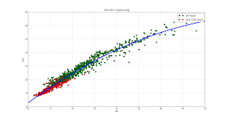
First, let's take a look at the VIX-VXV relationship:

The chart above shows VIX-VXV data since January 2010. Data points from last year are shown in red.
I have chosen to use a quadratic fit between the two, approximating VXV =  f(VIX) . The f(VIX) is plotted as a blue line.
The values above the line represent situation when the futures are in stronger than normal contango. Now I define a delta indicator, which is the deviation from the fit: delta = VXV-f(VIX).

Now let's take a look at the price of VXX along with delta:


Above: price of VXX on log scale. Below: delta. Green markers indicat delta > 0 , red markers delta<0.
It is apparent that green areas correspond to a negative returns in the VXX.

Let's simulate a strategy with this these assumptions:

  • Short VXX when delta > 0
  • Constant capital ( bet on each day is 100$)
  • No slippage or transaction costs
This strategy is compared with the one that trades short every day, but does not take delta into account.
The green line represents our VXX short strategy, blue line is the dumb one.

Metrics:
          Delta>0     Dumb
Sharpe:    1.9         1.2
Max DD:    33%         114% (!!!)

Sharpe of 1.9 for a simple end-of-day strategy is not bad at all in my opinion. But even more important is that the gut-wrenching drawdowns are largely avoided by paying attention to the forward futures curve.

Building this strategy step-by-step will be discussed during the coming Trading With Python course. 


Getting short volume from BATS

In my last post I have gone through the steps needed to get the short volume data from the BATS exchange. The code provided was however of the quick-n-dirty variety. I have now packaged everything to bats.py module that can be found on google code. (you will need the rest of the TradingWithPython library to run bats.py)

Usage:

import tradingWithPython as twp # main library
import tradingWithPython.lib.bats as bats # bats module

dl = bats.BATS_Data('C:\\batsData') # init with directory to save data
dl.updateDb() # update data
s = dl.loadData() # process zip files


Thursday, August 15, 2013

Building an indicator from short volume data

Price of an asset or an ETF is of course the best indicator there is, but unfortunately there is only only so much information contained in it. Some people seem to think that the more indicators (rsi, macd, moving average crossover etc) , the better, but if all of them are based at the same underlying price series, they will all contain a subset of the same limited information contained in the price.
We need more information additional to what is contained the price to make a more informed guess about what is going to happen in the near future. An excellent example of combining all sorts of info to a clever analysis can be found on the The Short Side of Long blog. Producing this kind of analysis requires a great amount of work, for which I simply don't have the time as I only trade part-time.
So I built my own 'market dashboard' that automatically collects information for me and presents it in an easily digestible form. In this post I'm going to show how to build an indicator based on short volume data. This post will illustrate the process of data gathering and processing.

Step 1: Find data source. 
BATS exchange provides daily volume data for free on their site.

Step 2: Get data manually & inspect
Short volume data of the BATS exchange is contained in a text file that is zipped. Each day has its own zip file. After downloading and unzipping the txt file, this is what's inside (first several lines):

Date|Symbol|Short Volume|Total Volume|Market Center
20111230|A|26209|71422|Z
20111230|AA|298405|487461|Z
20111230|AACC|300|3120|Z
20111230|AAN|3600|10100|Z
20111230|AAON|1875|6156|Z
....

In total a file contains around 6000 symbols.
This data is needs quite some work before it can be presented in a meaningful manner.

Step 3: Automatically get data
What I really want is not just the data for one day, but a ratio of short volume to total volume for the past several years, and I don't really feel like downloading 500+ zip files and copy-pasting them in excel manually.
Luckily, full automation is only a couple of code lines away:
First we need to dynamically create an url from which a file will be downloaded:

from string import Template

def createUrl(date):
    s = Template('http://www.batstrading.com/market_data/shortsales/$year/$month/$fName-dl?mkt=bzx')
    fName = 'BATSshvol%s.txt.zip' % date.strftime('%Y%m%d')
    
    url = s.substitute(fName=fName, year=date.year, month='%02d' % date.month)
    
    return url,fName
    
Output:
http://www.batstrading.com/market_data/shortsales/2013/08/BATSshvol20130813.txt.zip-dl?mkt=bzx

Now we can download multiple files at once:

import urllib

for i,date in enumerate(dates):
    source, fName =  createUrl(date)# create url and file name
    dest = os.path.join(dataDir,fName) 
    if not os.path.exists(dest): # don't download files that are present
        print 'Downloading [%i/%i]' %(i,len(dates)), source
        urllib.urlretrieve(source, dest)
    else:
        print 'x',

Output:
Downloading [0/657] http://www.batstrading.com/market_data/shortsales/2011/01/BATSshvol20110103.txt.zip-dl?mkt=bzx
Downloading [1/657] http://www.batstrading.com/market_data/shortsales/2011/01/BATSshvol20110104.txt.zip-dl?mkt=bzx
Downloading [2/657] http://www.batstrading.com/market_data/shortsales/2011/01/BATSshvol20110105.txt.zip-dl?mkt=bzx
Downloading [3/657] http://www.batstrading.com/market_data/shortsales/2011/01/BATSshvol20110106.txt.zip-dl?mkt=bzx

Step 4. Parse downloaded files

We can use zip and pandas libraries to parse a single file:
import datetime as dt
import zipfile
import StringIO

def readZip(fName):
    zipped = zipfile.ZipFile(fName) # open zip file 
    lines = zipped.read(zipped.namelist()[0]) # unzip and read first file 
    buf = StringIO.StringIO(lines) # create buffer
    df = pd.read_csv(buf,sep='|',index_col=1,parse_dates=False,dtype={'Date':object,'Short Volume':np.float32,'Total Volume':np.float32}) # parse to table
    s = df['Short Volume']/df['Total Volume'] # calculate ratio
    s.name = dt.datetime.strptime(df['Date'][-1],'%Y%m%d')
    
    return s

It returns a ratio of Short Volume/Total Volume for all symbols in the zip file:
Symbol
A         0.531976
AA        0.682770
AAIT      0.000000
AAME      0.000000
AAN       0.506451
AAON      0.633841
AAP       0.413083
AAPL      0.642275
AAT       0.263158
AAU       0.494845
AAV       0.407976
AAWW      0.259511
AAXJ      0.334937
AB        0.857143
ABAX      0.812500
...
ZLC       0.192725
ZLCS      0.018182
ZLTQ      0.540341
ZMH       0.413315
ZN        0.266667
ZNGA      0.636890
ZNH       0.125000
ZOLT      0.472636
ZOOM      0.000000
ZQK       0.583743
ZROZ      0.024390
ZSL       0.482461
ZTR       0.584526
ZTS       0.300384
ZUMZ      0.385345
Name: 2013-08-13 00:00:00, Length: 5859, dtype: float32


Step 5: Make a chart:

Now the only thing left is to parse all downloaded files and combine them to a single table and plot the result:


In the figure above I have plotted the average short volume ratio for the past two years. I also could have used a subset of symbols if I wanted to take a look at a specific sector or stock. Quick look at the data gives me an impression that high short volume ratios usually correspond with market bottoms and low ratios seem to be good entry points for a long position.

Starting from here, this short volume ratio can be used as a basis for strategy development.

Sunday, March 17, 2013

Trading With Python course - status update

I am happy to announce that a sufficient number of people have showed their interest in taking the course. This means that the course will definitely take place.
Starting today I will be preparing a new website and material for the course, which will start in the second week of April.

Thursday, January 12, 2012

Reconstructing VXX from CBOE futures data

Many people in the blogsphere have reconstructed the VXX to see how it should perform before its inception. The procedure to do this is not very complicated and well-described in the VXX prospectus and on the Intelligent Investor Blog. Doing this by hand however is a very tedious work, requiring to download data for each future separately, combine them in a spreadsheet etc.
The scripts below automate this process. The first one, downloadVixFutures.py , gets the data from cboe, saves each file in a data directory and then combines them in a single csv file, vix_futures.csv
The second script reconstructVXX.py parses the vix_futures.csv, calculates the daily returns of VXX  and saves results to reconstructedVXX.csv.
To check the calculations, I've compared my simulated results with the SPVXSTR index data, the two agree pretty well, see the charts below.

Note: For a fee, I can provide support to get the code running or create a stand-alone program, contact me if you are interested.


--------------------------------source codes--------------------------------------------

Code for getting futures data from CBOE and combining it into a single table
downloadVixFutures.py

#-------------------------------------------------------------------------------
# Name:        download CBOE futures
# Purpose:     get VIX futures data from CBOE, process data to a single file
#
#
# Created:     15-10-2011
# Copyright:   (c) Jev Kuznetsov 2011
# Licence:     BSD
#-------------------------------------------------------------------------------
#!/usr/bin/env python


from urllib import urlretrieve
import os
from pandas import *
import datetime
import numpy as np

m_codes = ['F','G','H','J','K','M','N','Q','U','V','X','Z'] #month codes of the futures
codes = dict(zip(m_codes,range(1,len(m_codes)+1)))

dataDir = os.path.dirname(__file__)+'/data'


def saveVixFutureData(year,month, path, forceDownload=False):
    ''' Get future from CBOE and save to file '''
    fName = "CFE_{0}{1}_VX.csv".format(m_codes[month],str(year)[-2:])
    if os.path.exists(path+'\\'+fName) or forceDownload:
        print 'File already downloaded, skipping'
        return
    
    urlStr = "http://cfe.cboe.com/Publish/ScheduledTask/MktData/datahouse/{0}".format(fName)
    print 'Getting: %s' % urlStr
    try:
        urlretrieve(urlStr,path+'\\'+fName)
    except Exception as e:
        print e

def buildDataTable(dataDir):
    """ create single data sheet """
    files = os.listdir(dataDir)

    data = {}
    for fName in files:
        print 'Processing: ', fName
        try:
            df = DataFrame.from_csv(dataDir+'/'+fName)
            
                    
            code = fName.split('.')[0].split('_')[1]
            month = '%02d' % codes[code[0]]
            year = '20'+code[1:]
            newCode = year+'_'+month
            data[newCode] = df
        except Exception as e:
            print 'Could not process:', e
        
        
    full = DataFrame()
    for k,df in data.iteritems():
        s = df['Settle']
        s.name = k
        s[s<5] = np.nan
        if len(s.dropna())>0:
            full = full.join(s,how='outer')
        else:
            print s.name, ': Empty dataset.'
    
    full[full<5]=np.nan
    full = full[sorted(full.columns)]
        
    # use only data after this date
    startDate = datetime.datetime(2008,1,1)
    
    idx = full.index >= startDate
    full = full.ix[idx,:]
    
    #full.plot(ax=gca())
    print 'Saving vix_futures.csv'
    full.to_csv('vix_futures.csv')


if __name__ == '__main__':

    if not os.path.exists(dataDir):
         print 'creating data directory %s' % dataDir
         os.makedirs(dataDir)

    for year in range(2008,2013):
        for month in range(12):
            print 'Getting data for {0}/{1}'.format(year,month+1)
            saveVixFutureData(year,month,dataDir)

    print 'Raw wata was saved to {0}'.format(dataDir)
    
    buildDataTable(dataDir)

Code for reconstructing the VXX
reconstructVXX.py
"""
Reconstructing VXX from futures data

author: Jev Kuznetsov

License : BSD
"""
from __future__ import division
from pandas import *
import numpy as np

class Future(object):
    """ vix future class, used to keep data structures simple """
    def __init__(self,series,code=None):
        """ code is optional, example '2010_01' """
        self.series = series.dropna() # price data
        self.settleDate = self.series.index[-1]
        self.dt = len(self.series) # roll period (this is default, should be recalculated)
        self.code = code # string code 'YYYY_MM'
    
    def monthNr(self):
        """ get month nr from the future code """
        return int(self.code.split('_')[1])
         
    def dr(self,date):
        """ days remaining before settlement, on a given date """
        return(sum(self.series.index>date))
    
    
    def price(self,date):
        """ price on a date """
        return self.series.get_value(date)


def returns(df):
    """ daily return """
    return (df/df.shift(1)-1)


def recounstructVXX():
    """ 
    calculate VXX returns 
    needs a previously preprocessed file vix_futures.csv     
    """
    X = DataFrame.from_csv('vix_futures.csv') # raw data table
    
    # build end dates list & futures classes
    futures = []
    codes = X.columns
    endDates = []
    for code in codes:
        f = Future(X[code],code=code)
        print code,':', f.settleDate
        endDates.append(f.settleDate)
        futures.append(f)

    endDates = np.array(endDates) 

    # set roll period of each future
    for i in range(1,len(futures)):
        futures[i].dt = futures[i].dr(futures[i-1].settleDate)


    # Y is the result table
    idx = X.index
    Y = DataFrame(index=idx, columns=['first','second','days_left','w1','w2','ret'])
  
    # W is the weight matrix
    W = DataFrame(data = np.zeros(X.values.shape),index=idx,columns = X.columns)

    # for VXX calculation see http://www.ipathetn.com/static/pdf/vix-prospectus.pdf
    # page PS-20
    for date in idx:
        i =nonzero(endDates>=date)[0][0] # find first not exprired future
        first = futures[i] # first month futures class
        second = futures[i+1] # second month futures class
        
        dr = first.dr(date) # number of remaining dates in the first futures contract
        dt = first.dt #number of business days in roll period
        
        W.set_value(date,codes[i],100*dr/dt)
        W.set_value(date,codes[i+1],100*(dt-dr)/dt)
     
        # this is all just debug info
        Y.set_value(date,'first',first.price(date))
        Y.set_value(date,'second',second.price(date))
        Y.set_value(date,'days_left',first.dr(date))
        Y.set_value(date,'w1',100*dr/dt)
        Y.set_value(date,'w2',100*(dt-dr)/dt)
    
    
    valCurr = (X*W.shift(1)).sum(axis=1) # value on day N
    valYest = (X.shift(1)*W.shift(1)).sum(axis=1) # value on day N-1
    Y['ret'] = valCurr/valYest-1    # index return on day N

    return Y


##-------------------Main script---------------------------

Y = recounstructVXX()

print Y.head(30)#
Y.to_csv('reconstructedVXX.csv')


Monday, December 26, 2011

howto: Observer pattern

The observer pattern comes very handy when dealing with complex systems. It allows for class-to class communication with a very simple structure. Even more important is the ability to separate functionality in different modules, for example running a single 'broker' as a wrapper to some api and letting multiple strategies subscribe to relevant broker events. There are some ready-made modules available, but the best way to understand how this process works is to write the whole system from scratch. In many languages this is a very tedious task, but thanks to the power of Python it only takes a couple of lines to do this.

The following example code creates a Sender class (named Alice). Sender keeps track of interested listeners and notifies them accordingly. In more detail, this is achieved by a dictionary containing a function-event mapping, Sender.listeners.
A listener class can be of any type, here I make a bunch of ExampleListener classes, named Bob,Dave & Charlie. All of them have a method, that is that is subscribed to Sender. The only special thing about the subscribed method is that it should contain three parameters: sender, event, message. Sender is the class reference of the Sender class, so a listener would know who sent the message. Event is an identifier, for which I usually use a string. Optionally, a message is the data that is passed to a function.
A nice detail is that if a listener method throws an exception, it is automatically unsubscribed from further events.


'''
Created on 26 dec. 2011
Copyright: Jev Kuznetsov
License: BSD

sender-reciever pattern.

'''

import tradingWithPython.lib.logger as logger
import types

class Sender(object):
    """
    Sender -> dispatches messages to interested callables 
    """
    def __init__(self):
        self.listeners = {}
        self.logger = logger.getLogger()
        
        
    def register(self,listener,events=None):
        """
        register a listener function
        
        Parameters
        -----------
        listener : external listener function
        events  : tuple or list of relevant events (default=None)
        """
        if events is not None and type(events) not in (types.TupleType,types.ListType):
            events = (events,)
             
        self.listeners[listener] = events
        
    def dispatch(self,event=None, msg=None):
        """notify listeners """
        for listener,events in self.listeners.items():
            if events is None or event is None or event in events:
                try:
                    listener(self,event,msg)
                except (Exception,):
                    self.unregister(listener)
                    errmsg = "Exception in message dispatch: Handler '{0}' unregistered for event '{1}'  ".format(listener.func_name,event)
                    self.logger.exception(errmsg)
            
    def unregister(self,listener):
        """ unregister listener function """
        del self.listeners[listener]             
                   
#---------------test functions--------------

class ExampleListener(object):
    def __init__(self,name=None):
        self.name = name
    
    def method(self,sender,event,msg=None):
        print "[{0}] got event {1} with message {2}".format(self.name,event,msg)
                   

if __name__=="__main__":
    print 'demonstrating event system'
    
    
    alice = Sender()
    bob = ExampleListener('bob')
    charlie = ExampleListener('charlie')
    dave = ExampleListener('dave')
    
    
    # add subscribers to messages from alice
    alice.register(bob.method,events='event1') # listen to 'event1'
    alice.register(charlie.method,events ='event2') # listen to 'event2'
    alice.register(dave.method) # listen to all events
    
    # dispatch some events
    alice.dispatch(event='event1')
    alice.dispatch(event='event2',msg=[1,2,3])
    alice.dispatch(msg='attention to all')
    
    print 'Done.'


Wednesday, December 14, 2011

Plotting with guiqwt

While it's been quiet on this blog, but behind the scenes I have been very busy trying to build an interactive spread scanner. To make one, a list of ingredients is needed:

gui toolkit: pyqt -check.
data aquisition: ibpy & tradingWithPython.lib.yahooData - check.
data container: pandas & sqlite - check.
plotting library: matplotlib - ehm... No.

After tinkering with matplotlib in pyqt for several days I must admit its use in interactive applications is far from optimal. Slow, difficult to integrate and little interactivity. PyQwt proven to work a little better, but it had its own quirks, a little bit too low-level for me.
But as it often happens with Python, somebody, somewhere has already written a kick-ass toolkit that is just perfect for the job. And it looks like guiqwt is just it. Interactive charts are just a couple of code lines away now, take a look at an example here: Creating curve dialog . For this I used guiqwt example code with some minor tweaks.

And of course a pretty picture of the result:

...If only I knew how to set dates on the x-axis....

Friday, November 4, 2011

How to setup Python development environment

If you would like to start playing with the code from this blog and write your own, you need to setup a development environment first. I've already put a summary of tools and software packages on the tools page and to make it even easier, here are the steps you'll need to follow to get up and running:

1. Install PythonXY. : this includes Python 2.7 and tools Spyder, Ipython etc.
2. Install Tortoise SVN. This is a utility that you need to pull the source code from Google Code
3. Install Pandas (time series library)

This is all you need for now.
To get the code, use 'Svn Checkout' windows explorer context menu that is available after installing Tortoise SVN. Checkout like this (change Checkout directory to the location you want, but it should end with tradingWithPython):
If all goes well, the most recent version of the files will be downloaded. I'll be writing more code and improving current one, you'll be able to stay in sync with my code by using 'svn update' context menu.

The final step is to launch Spyder (through pythonXY launcher or start menu) and add the directory just above the 'tradingWithPython' (in my example C:\Users\jev\Desktop') dir to python path . Do this with 'tools'->'PYTHONPATH manager'.
Ok, all done, now you can run the examples from \cookbok dir.

Friday, October 28, 2011

kung fu pandas will solve your data problems

I love researching strategies, but sadly I spend too much time on low-level work like filtering and aligning datasets. In fact, about 80% of my time is spent on this mind numbing work. There had got to be a better way than hacking all the filtering code myself, and there is!
Some time ago I've come across a data analysis toolkit pandas especially suited for working with financial data. After just scratching the surface of its capabilities I'm already blown away by what it delivers. The package is being actively developed by Wes McKinney  and his ambition is to create the most powerful and flexible open source data analysis/manipulation tool available. Well, I think he is well on the way!

Let's take a look at just how easy it is to align two datasets:

from tradingWithPython.lib import yahooFinance

startDate = (2005,1,1)

# create two timeseries. data for SPY goes much further back
# than data of VXX
spy = yahooFinance.getHistoricData('SPY',sDate=startDate)
vxx = yahooFinance.getHistoricData('VXX',sDate=startDate)

# Combine two datasets
X = DataFrame({'VXX':vxx['adj_close'],'SPY':spy['adj_close']})

# remove NaN entries
X= X.dropna()
# make a nice picture
X.plot()

Two lines of code! ( this could be even fit to one line, but I've split it for readability)
Here is the result:

Man, this could have saved me a ton of time! But it still will help me in the future, as I'll be using its DataFrame object as a standard in my further work.